Artificial Neurons

If you are not living under a rock you might have heard about artificial neural networks (ANNs).

This post is the first of a series in which I will introduce to the basic maths and concepts of ANNs and machine learning, possibly reaching the more advanced topics of this fascinating discipline while keeping things simple and clear (hopefully).

The starting episode is therefore devoted to the building blocks of any neural network: the neurons.

Perceptrons

The first type of artificial neuron, called perceptron was developed in the 60s by the scientist Frank Rosenblatt inspired by earlier work by Warren McCulloch and Walter Pitts. Nowadays it’s more common to use other models of artificial neurons such as the sigmoid neurons whose properties will be described later once we understand how perceptrons works.

Perceptrons are quite simple objects which takes several binary inputs, $x_1$, $x_2$, …, and produce one binary output, \(o\):

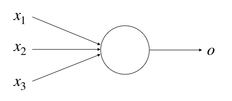
The simple approach proposed by Rosenblatt to compute the output was by introducing weights, $w_1$, $w_2$, …, real numbers expressing the importance of the respective inputs to the output. The neuron’s output, 0 or 1, is determined by whether the weighted sum $\sum_{j} w_j x_j$ is less than or greater than some threshold value which, just like the weights, is another real number.

To put it in a more formal way:

And that is basically everything we have to say from a mathematical point of view about perceptrons !

We can be a little bit more fancy and simplify the notation by rewriting the weighted sum as a dot product, $\sum_{j} w_j x_j = w \cdot x$ where $w$ and $x$ are vectors whose components are the weights and inputs, respectively. Also we can move the threshold on the other side of the inequality and replace it by what’s known as the perceptron’s bias, $b \equiv - \text{threshold}$.

Eq. 1 becomes:

You can think of the bias as a measure of how easy it is to get the perceptron to output a 1. Or, to put it in more biological terms, the bias is a measure of how easy it is to get the perceptron to fire. A perceptron with a really large positive bias would easily output a 1. On the other hand, if the bias is a very large negative number, then it would be difficult for the perceptron to output a 1. Obviously, introducing the bias is only a small change in how we describe perceptrons, but we’ll see later on that it leads to further notational simplifications.

To make a trivial example, let us consider the perceptron in Fig. 1 with 3 inputs. The output for a 3-inputs perceptron can be calculated using Eq. 2, explicitly:

where $ * $ is the classic multiplication operator.

Let’s say that the output is whether you go ($o = 1$) or not ($o = 0$) to a music festival based on:

1. your favourite band is playing ($x_1 = 1$) or not ($x_1 = 0$)
2. your friends are coming ($x_2 = 1$) or not ($x_2 = 0$)
3. it is sunny ($x_3 = 1$) or not ($x_3 = 0$)

If the most important thing for you is the band playing followed by your friends coming while you don’t care about the weather, the perceptron which best model this kind of decision-making would have for example $w_1 = 6$, $w_2 = 4$ and $w_3 = 0$. Finally, let’s say that this perceptron has a threshold of 5 (bias, $b = -5$). For this choice that means that you will go to the concert ($o = 1$) whenever your favourite band is playing and it actually doesn’t matter if your friends are coming or if it is sunny (just use Eq. 3 to check it).

By varying the weights and bias we can get different models of decision-making. Let’s say for example that the bias is $b = -4$ (i.e. you’re more inclined to go to the the concert, in general): in this case you will go to the concert if your favourite band is playing or if your friend are coming (or both), regardless of the atmospheric conditions.

Perceptrons are therefore a tool for decision making but they can also be used to compute basic logic functions such as AND, OR and NAND. For example, let’s suppose we have a perceptron with two inputs ($x_1$ and $x_2$), each with weight −2 ($w_1 = w_2 = -2$), and an overall bias of 3 ($b = 3$). Using Eq. 3 we can easily verify that an input 00 ($x_1 = x_2 = 0$) will produce an output $o = 1$. The same happens for an input 01 and 10 while for an input 11 the output will be 0. This perceptron therefore implements a NAND gate. Those familiar with Boolean functions and logic have already grasped the importance of it, being the NAND gate functionally complete, i.e. any logical function can be obtained using only NAND gates.

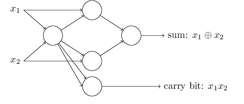
A classic example in digital electronics is to use only NAND gates to build a circuit to add 2 bits $x_1$ and $x_2$, as shown in Fig. 2.

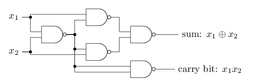
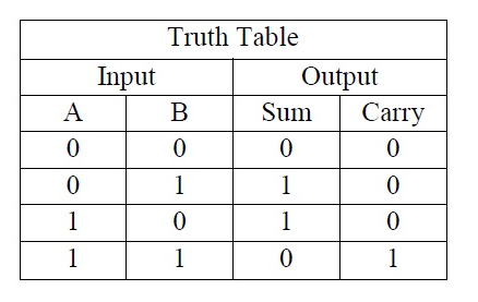
where the carry bit is set to 1 when both $x_1$ and $x_2$ are equal to 1. The truth table for the half adder is shown in Fig. 3.

The corresponding “2-bits-adder-network” using the “NAND-perceptrons” described above will look like the one showed in Fig. 4.

You might have noticed that the leftmost perceptron’s output is used twice as an input for the bottom-right perceptron. In principle nothing forbid this kind of behaviour but if we don’t like it we could just merge the two lines in a single connection with weight -4 to obtain the same result (it’s up to you to verify it). Also, up to now we showed the inputs as variables floating to the left of the network but conventionally they are represented as perceptrons in what is called the input layer. Input neurons have one output but no input. In fact they are not really neurons but this representation makes neural networks look prettier. The nicer version of our half adder network is shown in Fig. 5

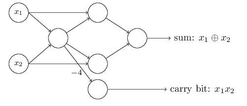
where all perceptrons have a weights $w_1 = w_2 = -2$ and bias $b=3$ with the exception of the bottom right perceptron which has an explicitly indicated weight of -4. You may have noticed also that in the network depicted in Fig. 5 we have some layers of neurons in between the input and the output. These “in-between” layers are conventionally referred as hidden layers. Neurons composing the hidden layers are no different from any other neuron and the term basically means “not an input nor an output”. While the design of the input and output layers of a neural network is often straightforward, there can be quite an art to the design of the hidden layers. In particular, it’s not possible to sum up the design process for the hidden layers with a set of simple rules. Instead, neural networks researchers have developed many design heuristics for the hidden layers, which help people get the behaviour they want out of their nets. For example, such heuristics can be used to help determine how to trade off the number of hidden layers against the time required to train the network. As a rule of thumb one may consider to add hidden layers to introduce complexity because what they do, mathematically speaking, is performing nonlinear transformations of the inputs entered into the network.

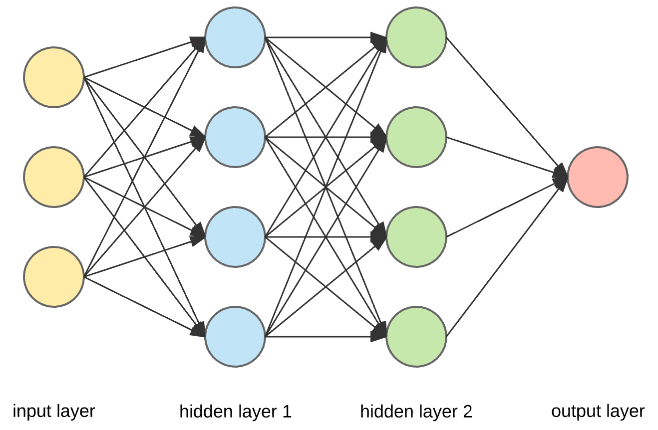
A conventional architecture for an ANN might look like the one showed in Fig. 6.

Because NAND gates are universal for computation, the adder example demonstrate that perceptrons are universal too. This is both reassuring and disappointing: are perceptrons just another type of NAND gates ? Of course not and they are much more than this because it turns out that we can devise learning algorithms which can automatically tune the weights and biases of a network of artificial neurons. This tuning happens in response to external stimuli, without direct intervention by a programmer. These learning algorithms enable us to use artificial neurons in a way which is radically different to conventional logic gates. Instead of explicitly laying out a circuit of NAND and other gates, our neural networks can simply learn to solve problems, sometimes problems where it would be extremely difficult to directly design a conventional circuit.

Learning algorithms and how ANNs actually work will be the topic of future posts of this series. However, in order to work, these algorithms need to tunes the parameters of a different kind of neurons capable of accepting as inputs and producing as output any number between 0 and 1 and not just 0 or 1.

Sigmoids

Even without any detailed explication on how learning algorithms operate, a problem instantly arise with perceptrons: if these algorithms can effectively fine tune the weights and biases of the artificial neurons, one might expect that a small change will lead to a small change in the final output. With perceptrons that’s not the case because the output, which is binary, will be 0 until it becomes 1, and viceversa. As anticipated at the beginning, perceptrons are not used nowadays in neural network and the reason is the one just mentioned: a small changes in the weights and bias can lead to a completely different output. For this reason other neurons are used in ANNs such as the sigmoid neuron.

Just like a perceptron, the sigmoid neuron has inputs, $x_1$, $x_2$,… But instead of being just 0 or 1, these inputs can take on any values between 0 and 1. So, for instance, 0.683… is a valid input for a sigmoid neuron. Also, just like a perceptron, the sigmoid neuron has weights for each input, $w_1$, $w_2$,…, and an overall bias, $b$, but the output is not 0 or 1. Instead, it’s $\sigma(w \cdot x + b)$, where $\sigma$ is the sigmoid function defined as:

where $z = w \cdot x + b$.

For a sigmoid neuron with $x_1$, $x_2$,…, weigths $w_1$, $w_2$,…, and bias $b$ the output can be explicitly written as:

It seems that sigmoid neurons are a completely different beast with respect to perceptrons but they are not, actually. In order to understand the similarities and differences between the two it suffices to take a look at the shape of the sigmoid function:

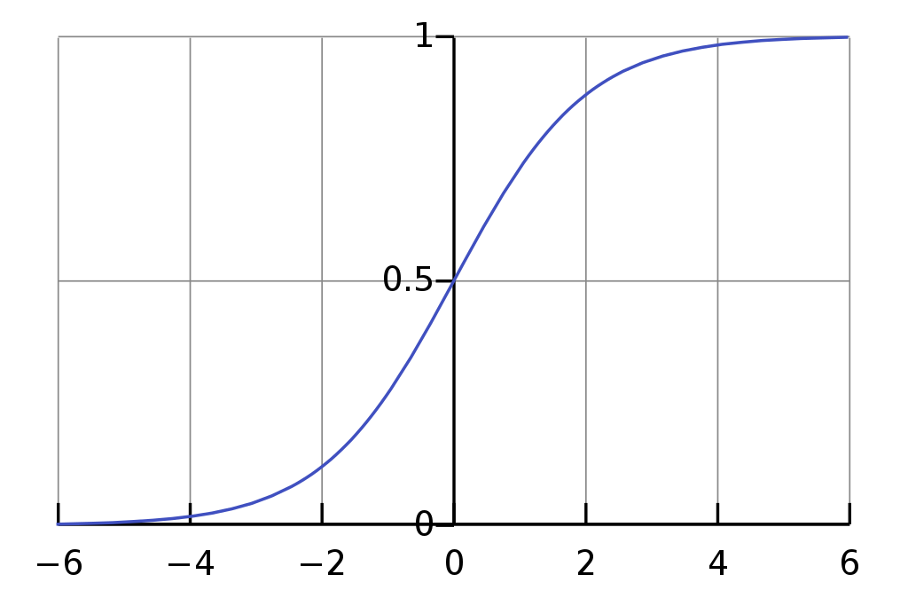
where $z$ on the x-axis belongs to the interval $(-\infty, \infty)$ and $\sigma(z)$ on the y-axis belongs to the interval $(0, 1)$.

We have seen before that when the bias, and therefore $z$, is large and positive, a perceptron will fire ($o = 1$) while if $z$ is a very large and negative number the perceptron’s output will be 0. If you look at Fig.6 you will notice that for these extreme cases it behaves the same: the sigmoid function “squeezes” very large negative numbers to 0 and very large positive number to 1. The main and most important difference is that it’s able to transit from 0 to 1 smoothly and outputting values between 0 and 1 when the absolute value of $z$ is not very large.

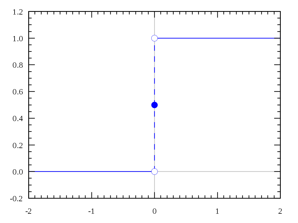
Turning around to this point of view, it’s like if the perceptron output was described by the step function, shown in Fig.7 below (with the exception that when $z=0$ the perceptron outputs 0 while the step function outputs 1).

The sigmoid neuron can be considered as a smoothed perceptron and it is actualy the smoothness of the sigmoid function which plays a crucial role rather than it’s detailed form. The smoothness of $\sigma$ means that small changes $\Delta w_j$ in the weights and $\Delta b$ in the bias will produce a small change $\Delta output$ in the output from the neuron. In a more mathematical and formal way:

where the sum is over all weights, $w_j$, and $\partial output / \partial w_j$ and $\partial output / \partial b$ denote partial derivatives of the output with respect to $w_j$ and $b$, respectively. Even if you’re not familiar with partial derivatives and Eq. 6 looks really complicated, the only thing that it means is that $\Delta output$ is a linear function of the changes $\Delta w_j$ and $\Delta b$ in the weights and bias, which is really good news !

So, if it’s the shape of $\sigma$ which really matters and not its exact form, why choosing this function rather than another function (such as, for example, the arctangent) ? In fact, we will see that we can chose other functions and it is worth mentioning that these function “modulating” an artificial neuron’s output are called activation functions. The difference among activation functions and the art of choosing the most appropriate one, however, will be the topic of another post. In here, and in other simple examples you might find, the sigmoid function is the one used the most, mainly because exponentials have very lovely properties when differentiated and the algebra when calculating the pertial derivatives before (Eq. 6) is much easier with $\sigma$.

As a final (and trivial) note, how to interpret the real valued output of a sigmoid neuron ? If I want to classify an image as containing a cat or not, what $o = 0.234$ means ? Is it a cat or not ? One might establish a convention that if the value is below, let’s say 0.5, the answer is “no” while if it is above, it will be a “yes”. Otherwise, more interestingly, one can interpret the value as a probability value and therefore $o = 0.98$ will express more confidence that the image contains a cat with respect to an output $o = 0.68$.